Statistical Learning

What is statistial learning

Suppose we observe a quantitative response $Y$ and $p$ different predictors, $X_1, X_2, \ldots,X_p$ . We assume that there is a relationship between $Y$ and $X=(X_1, X_2,\ldots,X_p)$, which can be written as

$$ Y=f(X)+\epsilon $$

Here $f$ is some fixed but unknown fucntion of $X_1,X_2,\ldots,X_p$, and $\epsilon$ is a random error term, which is independent of $X$ and has mean zero. In this formulation, $f$ represents the systematic informationa $X$ provides about $Y$.

Why estimate $f$ ?

Two reasons: prediction and inference.

Prediction

In many cases, a set of input $X$ are readily available, but the output $Y$ can not be easily obtained. In this setting, since the error term averages to zero, we can predict $Y$ using

$$ \hat{Y} = \hat{f}(X) $$

Where $\hat{f}$ represents our estimate for $f$, and $\hat{Y}$ represents the resulting predictio for $Y$. In this setting, $\hat{f}$ is oftern treated as a black box, in the sense that one is not typically concerned with the exact form of $\hat{f}$, provided that it yields accurate predictions for $Y$.

reducible error and irreducible error

The accuray of $\hat{Y}$ as prediction for $Y$ depends on two quantities, which we will call them reducible error and irreducible error. In general, $\hat{f}$ will not be a perfect estimate for $f$, and this inaccuracy will introduce some error. This error is reducible because we can potentially improve the accuracy of $\hat{f}$ by using the most appropriate statistical learning techs to estimate $f$. However, even if it were possible to form a perfect etimate for $f$, so that our estimated response took the form $\hat{Y}=f(X)$, our prediction would still have some error in it!! Why? This is because $Y$ is also a function of $\epsilon$, which, by definition, cannot be predicted using $X$. Therefore, variables associated with $\epsilon$ also affects the accuracy of our predictions. This is known as the irreducible error.

Why is the irreducible error larger than zero? The quantify $\epsilon$ may contain unmeasured variables that are useful in predicting $Y$: since we don’t measure them, $f$ cannot use them for its prediction. The euatity $\epsilon$ may also contain unmeasurable variation. For example, the risk of an adverse reaction might vary for a given patient on a given ay, depending on manufacturing variation in the drug itself or the patient’s general feeling of well-being on that day.

Consider a given estimate $\hat{f}$ and a set of predictors $X$, which yields the prediction $\hat{Y}=\hat{f}(X)$. Assume for a moment that both $\hat{f}$ and $X$ are fixed. Then, it is easy to show that

$$ \begin{aligned} E(Y-\hat{Y})^2 &= E[f(X) + \epsilon - \hat{f}(X)]^2 \\ &=\underbrace{[f(X) - \hat{f}(X)]^2}_{reducible} + \underbrace{Var(\epsilon)}_{irreducible} \end{aligned} $$

Where $E(Y - \hat{Y})^2$ represents the average, or expected value, of the squared difference between the predicted and actual value of $Y$, and Var($\epsilon$) represents the variance associated with the error term $\epsilon$.

Keep in mind that the irreducible error will always provide an upper bound on hte accuracy of our prediction for $Y$. The focus would be estimating of $f$ with the aim of minimizing the reducible error.

Inference

We are often interested in understanding the way that $Y$ is affected as $X_1,X_2,\ldots,X_p$ change. In this situation we wish to estimate $f$, but our goal is not necessarily to make predictions for $Y$. We instead want to understand the relationship between $X$ and $Y$. More specifically, to understand how $Y$ changes as a function of $X_1,X_2,\ldots,X_p$.

Now $f$ cannot be treated as a black box, because we need to know its exact form. In this setting, one may be interested in answering the following questions:

Which predictors are associated with the response? It’s often the case that only a small fraction of the repdictors are substantially associated with $Y$. Identifying a few important predictors among a large set of possible variables can be very useful.
What is the relationship between the response and each predictor? Some predictors may have a positive relationship with $Y$, while others may have opposite relationships. Depending on the complexity of $f$, the relationship between the response and a given predictor may also depend on the valurs of the other predictors.
Can the relationship between $Y$ and each predictor be adequately summarized using a linear equation, or is the relatioship more complicated? Historically, most mthods for estimating $f$ have taken a linear form. In some situations, such an assumption is resonable or even desirable. But often the true relationship is more complicated, in which case a linear model may not provide an accurate representation of the relationship between the input and output variables.

How do we estimate $f$ ?

We will explore many linear and non-linear approaches for estimating $f$. However, these methods generally share certain characteristics.

Training data, data that will be used to train, or teach, our method how to estimate $f$.

The goal is to apply a statistical learning method to the training data in order to estimate the unknown function $f$. In other words, we want to find a funtion $\hat{f}$ that $Y\approx\hat{f}(X)$ for any given observation $(X, Y)$.

Broadly speaking, most statitical learning methods for this task can be characterized as either parametric or non-parametric.

Parametric Methods

Parametric methods involve a two-step model-based approach.

First, we make an assumption about the functional form, or shape, of $f$. For example, one very simple assumption is that $f$ is linear in $X$:

$$ f(X)=\beta_{0} + \beta_{1}X_{1} + \beta_{2}X_{2} + \cdots+\beta_{p}X_{p} $$

This is linear model. Once we have assumed that $f$ is linear, the problem of estimation $f$ is greatly simplified. Instead of having to estimate an entirely arbitrary p-dimentional function $f(X)$, one only needs to estimate the p+1 coefficients $\beta$.

After a model has been selected, we need a procedure that uses the training data to fit or train the model. In the case of the linear model, we need to estimate the parameters $\beta{0}$ , $\beta{1}$ , $\ldots$ , $\beta_{p}$. That is, we want to find values of these parameters such that

$$ Y \approx \beta_{0} + \beta_{1}X_{1} + \beta_{2}X_{2} + \cdots + \beta_{p}X_{p} $$

The most common approach to fitting the model is refered to as (ordinary) least squares.

The model-based approach just described is refered to as parametric; it reduces the problem ofestimating $f$ down to one of the estimating a set of parameters. Assuming a parametric form for $f$ simplifies the problem of estimating $f$ because it is generally much easier to estimate a set of parameters, such as $\beta_0, \beta_1, \ldots, \beta_p$ in the linear model, than it is to fit an entirely arbitrary function $f$ . The potentil disadvantage of a parametric approach is that the model we choose will usually not match the true unknown form of $f$. If the chosen model is too far from the true $f$, then our estimate will be poor. We can try to address this problem by choosing flexible models that can fit many different possible functional forms for $f$. But in general, fitting a more flexible model requires estimating a greater number of parameters. These more comlex models can lead to phenomenon known as overfitting the data, which essentially means they folow the errors, or noise, too closely.

Non-parametric Methods

Non-parametric methods do not make explicit assumptions about the duncitonal forms of $f$. Instead they seek an estimate of $f$ that gets as close to the data points as possible without being too rough or wiggly.

Such approaches can have a major advantage over parametric approaches: by avoiding the assumption of a particular functional form for $f$, they have the potential to accurately fit a wider range of possible shapes for $f$.

Any parametric approach brings with it the possibility that the functional form used to estimate $f$ is very different from the true $f$, in which case the resulting model will not fit hte data well.

In contrast, non-parametric approaches completely avoid this danger, since essentially no assumption about the form of $f$ is mad. But non-parametric approaches do suffer from a major disadvantage: since they do not reduce the problem of estimating $f$ to a small number of parameters, a very large number of observations (far more than is typically needed for a parametric approace) is required in order to obtain and accurate estiamte for $f$.

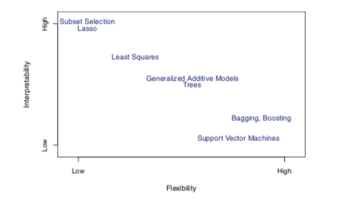
The Trade-Off between prediction accuracy and Model interpretability

More flexible model can generate a much wider range of possible shapes to estimate $f$. Why would we ever choose to use a more restrictive method instead of a very flexible approach? The more restrictive models are much more interpretable.

flexiblity

When inference is the goal, there are clear advantages to using simple and relatively inflexible statistical learning methods. In some seetings, however, we are only interested in prediciton and teh interpretability of the prediction model is simply not of interest. For exampl,e if we seek to develop an algorithm to predict the price of a stock, our sole requirement for the requirement for the algorithm to predict the price accurately – interpretability is not a concern. In this case, we might expect that it will be best to use the most flexible model available. Surprisely, this is not always the case! We will often obtain more accurate predictions using a less flexible method. This phenomenon, which may seem couterintuitive at first glace, has to do with the potential for overfitting in highly flexible methods.

Supervised VS Unsupervised Learning

Most statistical learning problems fall into one of the two categories: supervised or unsupervised.

Supervised: For each obervation of the predictor measurements $x_i, i=1,2,\ldots ,n$ there is an associated response measurement $y_i$. We wish to fit a model that relates the response to the predictors, with the aim of accurately predicting the response for future observations or better understanding the relationship between the response and the predictors. Many classical statistical learning methods such as linear regression and logistic regression, as well as more modern approaches such GAM, boosting, and support vector machines, operate in the supervised learning domain.

Unsupervised: in contrast, unserpervised learning describes the somewhat more challenging situation in which for every obervation $i=1,2,\ldots, n$, we observe a vector of measurements $x_i$ but no associated response $y_i$. It is not possible to fit a linear regression model, since there is no response variable to predict. In this setting, we are in some sense working blind; the situation is referred to as unsupervised because we we lack a response variable that can supervise our analysis. What sort of analysis is possible? cluster analysis, the goal of cluster analysis is to ascertain, on the basis of $x_1, \ldots, x_n$, whether the observations fall into relatively distinct groups.

Many problems fall naturally into the supervised or unsupervised learning paradigms. However, sometimes the question of whether an analysis shoudl be considered supervised or unsupervised is less clear-cut. For instance, suppose that we have a set of $n$ observations. Fomr $m$ of hte observations, where $m < n$, we have both predictor measurements and a response measurement. For the remaining $n - m$ obervations, we have predictor measurements but no response measurement. SUch a scenario can arise if the predictors can be measured relatively cheaplly but hte corresponding response are much more expensive to collect. We reger to this setting as a semi-supervised learning problem. In this setting, we wish to use a statistical learning method that can incorporate the $m$ obervations for which response measurements are available as well as the $n-m$ observations for which they are not.

Regression VS Classification problems

Variables can be characterized as either quantitative or qualitative (also known as categorical). We tend to refer to problems with a quantitative response as regression problems, which those involving a qualitative response are ofter refered to as classification problems. However, the distinction is not always that crisp. Least squares linear regression is used with a quantitative response, whereas logistic regression is typically used with a qualitative (two-class, or binary) response. As such it is oftern used as a classification method. But since it estimates class probabilities, it can be thought of as a regression method as well. Some statistical methods, such as K-nearest neighbors and boosting, can be used in the case of either quantitative or qualitative responses.

We tend to select statistical learning methods on the basis of whether the response is quantitative or qualitative; i.e. we might use linear regression when quantitative and logistic regression when qualitative. However, whether the predictors are qualitative or quantitative is gneerally condisered less important. Most of the statistical learning methods can be applied regardless of the predictor variable type, provided that any qualitative predictors are properly coded begore the analysis is performed.

Assessing Model Accuracy

There is no free lunch in statistics: no one method dominates all others over all possible data sets. Hence it is important to decie for any given set of data which method produces the best results. Selecting the best approach can be one of the most challenging parts of performing statistical learning in practice.

Measuring the quality of Fit

In order to evaluate the performance of a statistical learning method on a given data et, we need some way to meaure how well its predictions actually match the observed data. That is. we need to quantify the extent to which the predicted response value for a given observation is close to the true response value for that observation. In the regression settting, the most commonly-used measure is the mean squared error (MSE), given by

$$ MSE=\frac{1}{n}\sum_{j=0}^n (y_i-\hat{f}(x_i))^2 $$

The MSE is computed using the training data that was used to fit the model, and so should more accurately be refered to as the training MSE. But in general, we do not really care how well the method works on the training data. Rather, we are interested in the accuracy of the predictions that we obtain when we apply our method to previously unseen test data. Why? Think about training model to predict stock price.

Suppose that we fit our statistical learning method on our training observations ${(x_1, y_1), (x_2, y_2), \ldots, (x_n, y_n)}$, and we obtain the estimate $\hat{f}$. We can then compute $\hat{f}(x_1), \hat{f}(x_2), \ldots. \hat{f}(x_n)$. If these are approximately equal to $y_1,y_2,\ldots,y_n$, then the training MSE is small. However, we are really not interested in whether $\hat{f}(x_i) \approx y_i$; instead, we want to know where $\hat{f}(x_0)$ is approximately equal to $y_0$, where $(x_0, y_0)$ is a previously unseen test observation not used to train the statistical learning method.

We want to choose the method that gives the lowest test MSE, as opposed to the lowest training MSE. In other words, if we had a large number of test observations, we could compute

$$ Ave(y_0 - \hat{f}(x_0))^2 $$

The average square prediction error for these test observations $(x_0, y_0)$.

The Bias-Variation Trade-Off

For a given value $x_0$, the expected test MSE can be decomposed into the sum of three fundamental quantities: the variance of $\hat{f}(x_0)$, the squared bias of $\hat{f}(x_0)$ and the variance of the error term $\epsilon$. That is

$$ E(y_0 - \hat{f}(x_0))^2 = Var(\hat{f}(x_0)) + [Bias(\hat{f}(x_0))]^2 + Var(\epsilon) $$

Here the notation $E(y_0-\hat{f}(x_0))^2$ defines the exptected test MSE, and refers to the average test MSE that we would obtain if we repeatedly estimated $f$ using a large number of training sets, and tested each at $x_0$. The overall expected test MSE can be computed by averaging $E(y_0-\hat{f}(x_0))^2$ overall possible values of $x_0$ in the test set.

The equation shows that in order to minimize the expected test error, we need to select a statistical learning method that simultaneously achieves low variance and low bias.

What do we mean by the the variance and bias of a statistical learning method?

Variance referes to the amount of by which $\hat{f}$ would change if we estimated it using a different training data set. Since the training data are used to fit the statistical method, different training data sets will result in a different $\hat{f}$. But ideally the estimate of $f$ should not vary too much between training sets.

If a method has high variance then small changes in the training data can result in large changes in $\hat{f}$. In general, more flexible statistical methods have higher variance.

Bias referes to theerro that is introduced by approximating a real-life problem, which may be extremely complicated, by as much simpler model.

As a general ruls, as we use more flexible methods, the variance will increase and the bias will decrease.

The Classification Setting

Suppose that we seek to estimate $f$ on the basis of training observations ${(x_1, y_1), \ldots, (x_n, y_n)}$, where now $y_1,\ldots,y_n$ are qualitative. The training error rate is calculated as the proportion of mistakes that are made if we apply our estimte $\hat{f}$ to the training observations:

$$ \frac{1}{n}\sum_{i=1}^n I(y_i \neq \hat{y}_0) $$

Here $\hat{y}_i$ is the predicted class label for the ith observation using $\hat{f}$. And $I(y_i \neq \hat{y}_i)$ is an indicator variable that equals 1 if $y_i \neq \hat{y}_i$ and zero if $y_i = \hat{y}_i$.

As in the regression setting, we are most interested in the error rates that result from applying our classifier to test observations that were not used in training. The test error rate associated with a set of test observations of the form $(x_0, y_0)$ is given by

$$ Ave(I(y_0 \neq \hat{y}_0)) $$

The Bayes Classifier

To minimize the test error rate: assign each observation to the most likely class given its predictor values.

The conditional probability:

$$ Pr(Y=j|X=x_0) $$

It is the probability that $Y = j$, given the observed predictor vector $x_0$. This very simple classifier is called the bayes classifier.