In the regression setting, the standard linear model
is commonly used to describe the relationship between a response $Y$ and a set of variables $X_1, X_2, \ldots, X_p$. We have seen in Chapter 3 that one typiclaly fits this model using least square.
In the chapters that follow, we consider some approaches for extending the linear model framework. In chapter 7 we generalize (6.1) in order to accommodate non-linear, but still additive, relationships, while in Chapter 8 we consider even more general non-linear models. However, the linear model has distinct advantages in terms of inference and , on real-world problems, is oftern surprisingly competetive in relation to non-linear methods.
In this chapter, we discuss some ways in which the simple linear model can be improved, by replacing plain least squares fitting with some alternative fitting procedures.
Why might we want to use another fitting procedure instead of least squares? As we will see, alternative fitting procedures can yield better prediction accuracy and model interpretability.
Prediction accuracy: Provided that the true relationship between the response and the predictors is approximately linear, the least squares estimates will have low bais. If $n \gg p$, that is if $n$, the number of observations, is much larger than $p$, the number of variables, then the least squares estimates tend to also have low variance, and hence will perform well on test observations. However, if $n$ is not much larger than $p$, then tere can be a lot of variability in the least squares fit, resulting in overfitting and consequently poor predictions on future observationss not used in the model training. And if $p > n$, then there is no longer a unique least saures coefficient estimate: the variance if infinite so the method cannot be used at all. By
constrainingorshrinkingthe estiamted coefficients, we can oftern substantially reduce the variance at the cost of negligible increase in bias. This can lead to substantial improvements in the accuracy with which we can predict the response for observations not used in the model training.Model Interpretability: It is often the case that some or many of the variables used in a multiple regression model are in fact not associated with the response. Including such
irrelavantvariables leads to unnecessary complexity in the resulting model. By removing these variables–that is, by setting the corresponding coefficient estimates to zero–we can obtain a model that is more easily interpreted. Now least squares i extremely unlikely to yield any coefficient estimates that are exactly zero. In this chapter, we see some approaches for automatically performingfeature selectionorvariable selection– that is, for excluding irrelevant variables from a multiple regression model.
There are many alternatives, both classical and modern, to using least squares to fit (6.1). In this chapter, we discuss three important classes of methods.
Subset Selection. This approach involves identifying a subset of the $p$ predictors that we believe to be related to the response. We then fit a model using least squares on the reduced set of variables.
Shrinkage. This appraoch involves fitting a model involving all $p$ predictors. However, the estimated coefficients are shrunken towards zero relatively to the least squares estimates. This shrinkage, also know as
regularization, has the effect of reducing variance. Depending on what type of shrinkage is performed, some of the coefficients may be estimated to be exactly zero. Hence, shrinkage methods can also perform variable selection.Dimension Reduction. This approach involves projecting the $p$ predictions into a M-dimentional subspace, where $M < p$. This is achieved by computing $M$ different
linear combinations, orprojections, of the variables. Then these $M$ projections are used as predictors to fit a linear regression model by least squares.
Subset Selection
Methods include best subset and stepwise model selection procedures.
Best Subset Selection
To perform best subset selection, we fit a separate least squares regression for each possible combination of the $p$ predictors. That is, we fit all $p$ models that contain exactly one predictors, all $\big(_2^p\big) = p(p-1)/2$ models that contain exactly two predictors, and so forth. We then look at all the resulting models, with the goal of identifying the one that is best.
This problem of selecting the best model among the $2^p$ possibilities considered by best subset selection is not trivial.
| Algorithm 6.1 Best subset selection |
|---|
| 1. Let $\Mu_0$ denote the null model, which contains no predictions. This model simply predicts the sample mean for each observaton. |
| 2. For $k = 1, 2, \ldots, p$: |
| 3. Select a single best model from among $\Mu_0,\ldots,\Mu_p$ using corss-validated prediction error, $C_p(AIC)$, $BIC$, or adjusted $R^2$. |
In Algorithm 6.1, Step 2 identifies the best model for each subset size, in order to reduce the problem from one of $2^p$ possible models to one of $p+1$ possible models.
Now in order to select a single a single best model, we must simply choose among the $p+1$ options. This task must be performed with care, because the RSS of these models decreases monotonically, and the $R^2$ increases monotonically, as the number of features included in the models increases. If we use these statistics to select the best model, then we will always end up with a model involving all of the variables. The problem is that a low RSS or high $R^2$ indicates a model with low training error, whereas we wish to choose a model that has a low test error. Therefore, in Step 3, we use corss-validated prediction error, $C_p$, BIC, or adjusted $R^2$ in order to seelct among $\Mu_0, \Mu_1, \ldots, \Mu_p$.
Although we have presented best subset selection here for least squares regression, the same ideas apply to other types of models, such as logistic regression. In the case of logistic regression, instead of ordering models by RSS in Step 2 of Algorithm 6.1, we instead use the deviance, a measure that plays the role of RSS for a broader class of models. The deviance, is negative two times the maximized log-likelihood; the smaller the deviance, the better the fit.
While best subset selection is a simple and conceptually appealing approach, it suffers fro computational limitations. Consuquently, best subset selection become cmoputationally infeasible for values of $p$ greater than 40, even with extremely fast modern computers.
Stepwise Selection
For computational reasons, best subset selection cannot be applied with very large $p$. Best subset selection may also suffer from statistical problems when $p$ is large: overfitting and high variance of the coefficient estimates.
For both of these reasons, stepwise method, which explore a far more restricted set of models, are attractive alternatives to best subset selection.
Forward Stepwise Selection
Forward stepwise selection begins with a model containing no predictors, and then adds predictors to the model, one-at-a-time, until all of the predictors are in the model. In particular, at each step the variable that gives the greatest additional improvement to the fit is added to the model. More formally, the forward stepwise selection procedure is given in Algorithm 6.2.
| Algorithm 6.2 Forward stepwise selection |
|---|
| 1. Let $\Mu_0$ denote the null model, which contains no predictors |
| 2. For $k=1,2,\ldots,p-1$: |
| 3. Select a single best model from among $\Mu_0,\ldots,\Mu_p$ using cross-validated prediction error, $C_p (AIC)$, BIC, or adjusted $R^2$ |
In Step 2(b) of Algorithm 6.2, we must identify the best model from among those $p-k$ that augment $\Mu_k$ with one additional predictor. We can do this by simply choosing the model with the lowest RSS or the highest $R^2$. However, in Step 3, we must identify the best model among a set of models with different number of variables. This is more challenging.
Forward stepwise selection’s computational advantage over best subset selection is clear. Though forward stepwise tend to do well in practice, it is not guaranteed to find the best possible model out of all $2^p$ models. For instance, suppose that in a given data set with $p=3$ predictors, the best possible one-variable model contains $X_1$, and the best possible two-variable model instead contains $X_2$ and $X_3$. Then forward stepwise selection will fail to select the best possible two-variable model, because $Mu_1$ will contain $X_1$, so $\Mu_2$ must also contain $X_1$ together with one additional variable.
Forward stepwise selection can be applied even in the high-dimensional setting where $n<p$; however, in this case, it is possible to construct submodels $\Mu_0,\ldots,\Mu_n-1$ only, since each submodel is fit using least squares, which wil not yield a unique solution if $p \ge n$.
Backward Stepwise Selection
Backward stepwise selection begins with the full least square model containing all $p$ predictors, and then iteratively removes teh least useful predictor, one-at-a-time.
| Algorithm 6.3 Backward stepwise selection |
|---|
| 1. Let $\Mu_p$ denote the full model, which contains all $p$ predictors. |
| For $k=p,p-1,\ldots,1$: |
| 3. Select the best model from among $\Mu_0,\ldots,\Mu_p$ using cross-validated prediction error, $C_p (AIC)$, BIC or adjusted $R^2$. |
Like forward stepwise selection, the backward selection approach searches through only $1+p(p+1)/2$ models, and so can be applied in settings where $p$ is too large to apply best subset selection. Also like forward selection, backward selection is not guaranteed to yield the best model containing a subset of the $p$ predictors.
Backward selection requires that the number of samples $n$ is larger than the number of variables $p$ (so that the full model can be fit). In contrast, forward stepwise can be used even when $n < p$, and so is the ony viable subset method when $p$ is very large.
Hybrid Approaches
The best subset, forward stepwise, and backward stepwise selection approaches generally give similar but not identical models. As an alternative, hybrid versions of forward and backward stepwise selection are available, in which variables are added to the model sequentially, in analogy to forward selection. However, after adding each new variable, the method may also remove any variables that no longer provide an improvement in the model fit. Such an approach attempts to more closely mimic best subset selection while retaining the computational advantages of forward and backward stepwise selection.
Choosing the Optimal Model
Best subset, forward and backward selection result in the creation of a set of models, each of which contains a subset of the $p$ predictors. In order to implement these methods, we need a way to determine which of these models is best. As we disscussed earlier, the model containing all of the predictors will always have the smallest $RSS$ and the largest $R^2$, since these these quantities are related to the training error. Instead, we wish to choose a model with a low test error. As we know, the training error can be a poor estimate of test error. Therefore, $RSS$ and $R^2$ are not suitable for selecting the best model among a collection of models with different numbers of predictors.
In order to select the best model with respect to test error, we need to estimate the test error. There are two common approaches:
We can indirectly estiamte test error by making an adjustment to the training error to account for the bias due to overfitting.
We can directly estiamte the test error, using either a validation set approach or a cross-validation approach.
$C_p, AIC, BIC$, and Adjusted $R^2$
Training set $RSS$ and training set $R^2$ cannot be used to select from among a set of models with different numbers of variables. However, a number of techniques for adjusting the training error for the model size are available. These approaches can be used to select among a set of models with different numbers of variables. We now consider four such approaches: $C_p$, Akaike information criterion (AIC), Bayesian information criterion (BIC), and adjusted $R^2$.
For a fitted least squares model containig $d$ predictors, the $C_p$ estimate of test MSE is computed using the equation
where $\hat{\sigma}^2$ is an estimate of the variance of the error $\epsilon$ associated with each response measurement in (6.1). Essentially, the $C_p$ statistic adds a penalty of $2d\hat{\sigma}^2$ to the training $RSS$ in order to adjust for the fact that the training error tends to underestimate the test error. Clearly, the penalty increases as the number of predictors in the model increases; this is intended to adjust for the corresponding decrease in training $RSS$.
The AIC criterion is defined for a large class of models fit by maximum likelihood. In the case of the model (6.1) with Gaussian errors, maximum likelihood and least squares are the same thing. In this case AIC is given by
where, for simplicity, we have omitted an additive constant. Hence for least squares models, $C_p$ and $AIC$ are proportional to each other.
BIC is derived froma Bayesian point of view, but ends up looking similar to $C_p$ and AIC. For the least squares model with $d$ predictors, the BIC is, up to irrelevant constants, given by
Like $C_p$, the BIC will tend to take on a small value for a model with a low test error, and so generally we select the model that has the lowest BIC value. Notice that BIC replaces the $2d\hat{\sigma}^2$ used by $C_p$ with a $log(n)d\hat{\sigma}^2$ term, where $n$ is the number of observations. Since $log(n) > 2$ for any $n > 7$, the BIC generally places a heavier penalty on models with many variables, and hence results in the selection of smaller models than $C_p$.
The adjusted $R^2$ statistic is another popular approach for selecting among a set of models that contain different numbers of variables. Recall from Chapter 3 that the usual $R^2$ is defined as $1 - RSS/TSS$, where$TSS - \sum(y_i-\bar{y})^2$ is the total sum of squares for the response. Since RSS always decreases as more variables are added, the $R^2$ always increases as more variables are added.
For a least squares model with $d$ variables, the adjusted $R^2$ statistic is calcualted as
Unlike $C_p$, $AIC$, and $BIC$, for which a small value indicates a model with a low test error, a large value of $adjusted \ R^2$ indicates a model with a small test error. Maximizing the $adjusted \ R^2$ is equivalent to minimizing $\frac{RSS}{n-d-1}$. While $RSS$ always decreases as the number of variables in the model increases, $\frac{RSS}{n-d-1}$ may increase or decrease, due to the presence of $d$ in the denominator.
$C_p$, $AIC$, and $BIC$ all have rigorous theoretical justifications. These justificatons rely on asymptotic arguments (scenarios where the sample size $n$ is very large). Despite its popularity, and even though it is quier intuitive, the adjusted $R^2$ is not as well motivated in statistical theory as $AIC$, $BIC$ and $C_p$. Here we have presented the formulas for $AIC$, $BIC$, and $C_p$ in the case of a linear model fit using least squares; however, these quantities can also be defined for more general types of models.
Validation and Cross-validation
As an alternative to the approaches just discussed, we can directly estimate the test error using the validation set and cross-validatoin methods. We can compute the validatoin set error or the cross-validation error for each model under consideration, and then select the model for which the resulting estiamted test error is smallest. This procedure has an adavantage realative to $AIC$, $BIC$, $C_p$ and adjusted $R^2$, in that it provides a direct estimate of the test error, and makes fewer assumptions about the true underlying model. It can also be used in a wider range of model selection tasks, even in cases where it is hard to pinpoint the model degree of freedom or hard to estimate the error varaince $\sigma^2$.
Shrinkage Methods
The subset selection methods described in Section 6.1 involve using least squares to fit a linear model that containts a subset of the predictors. As an alternative, we can fit a model containing all $p$ predictors using a technique that constrains or regularizes the coefficient estimates, or equivalently, that shrinks the coefficient estimates toward zero. It may not be immediately obvious why such a constraint should improve the fit, but it turns out that shrinking the coefficient estimates can significantly reduce their variance.
The two best-known techniques for shrinking the regression coefficients towards zero are ridge regression and the lasso.
Ridge Regression
Recall from Chapter 3 that the least squares fitting procedure estimates $\beta_0, \beta_1, \ldots,\beta_p$ using the values that minimize
Ridge regression is very similar to least squares, except that the coefficients are estimated by minimizing a slightly different quantity. In particular, the ridge regression coefficient estimates $\hat{\beta}^R$ are the values that minimize
where $\lambda \ge 0$ is a tuning parameter, to be determined separately. Equation 6.5 trades off two different criteria. As with least squares, ridge regression seeks coefficient estimates that fit the data well, by making the RSS small. However, the second term, $\lambda\Sigma_j\beta_j^2$, called a shrinkage penalty, is small when $\beta_1,\ldots,\beta_p$ are close to zero, and so it has the effect of shrinking the estimates of $\beta_j$ towards zero.
The tuning parameter $\lambda$ serves to control the relative impact of these two terms on the regression coefficient estimates. When $\lambda = 0$, the penalty term has no effect, and ridge regression will produce the least squares estimates. However, as $\lambda \rarr \inf$, the impact of the shrinkage penalty grows, and the ridge regression coefficient estimates will approach zero.
Unlike least squares, which generates only one set of coefficient estimates, ridge regression will produce a different set of coefficient estimates $\hat{\beta}_{\lambda}^R$, for each value of $\lambda$. Selecting a good value of $\lambda$ is critical.
Note that in (6.5), the shrinkage penalty is applied to $\beta_1,\ldots,\beta_p$, but not to the intercept $\beta_0$. We want to shrink the estiamted association of each variable with the response; however, we do not want to shrink the intercept, which is simply a measure of the mean value of the response.
The standard least squares coefficient estimates are scale equivariant: multiplying $X_j$ by a constant $c$ simply leads to a scaling of the least squares coefficient estimates by a factor of $1/c$. In other words, regardless of how the $j$th predictor is scaled, $X_j \hat{\beta}_j$ will remain the same. In contrast, the ridge regression coefficient estiamtes can change substantially when multiplying a given predictor by a constant. Therefore, it is best to apply ridge regression after standardizing the predictors, using the formula
so that they are all on the same scale. In (6.6), the denominator is the estimated standard deviation of the $j$th predictor. Consequently, all of the standardized predictors will have a standard deviation of one.
Why Does Ridge Regression Improve Over Least Squares
Ridge regression’s advantage over least squares is rooted in the bias-variance trade-off. As $\lambda$ increases, the flexibility of the ridge regression fit decreases, leading to decreased variance but increased bias. At the least squres coefficient estimates, which correspond to ridge regression with $\lambda = 0$, the variance is high but there is no bias. But as $\lambda$ increases, the shrinkage of the ridge coefficient estimates leads to a substantial reduction in the variance of the predictions, at the expense of a slight indrease in bias.
In general, in situations where the relationship between the response and the predictors is close to linear, the least squres estimates will have low bias but may have high variance. This means that a small change in the training data can cause a large change in the least squares coefficient estimates. In particular, when the number of variables $p$ is almost as large as the number of observations $n$. And if $p > n$, then the least squares estimates do not even have a unique solution, whereas ridge regression can still preform well by trading off a small increase in bias for a large decrease in variance. Hence, ridge regression works best in situations where the least squares estimates have high variance.
Ridge regression also have substantial computational advantages over best subset selection, which requires searching through $2^p$ models. As we discussed previously, even for moderate values of $p$, such a search can be computationally infeasible. In contrast, for any fixed value of $\lambda$, ridge regression only fits a single model, and the model-fitting procedure can be performed quite quickly.
The Lasso
Ridge regression does have one obvious disadvantages. Unlike best subset, foreward stepwise, and backward stepwise selection, which will generally select models that involve just a subset of the variables, ridge regression will include all $p$ predictors in the final model. The penalty $\lambda\Sigma\beta_j^2$ in (6.5) will shrink all of the coefficients toward zero, but it will not set any of them exactly to zero (unless $\lambda = \inf$). This may not be a problem for prediction accuracy, but it can create a challenge in model interpretation in settings in which the number of varaible $p$ is quite large.
The lasso is a relatively recent alternative to ridge regression that overcomes this disadvantage. The lasso coefficients, $\hat{\beta}_\lambda^L$, minimize the quantity
Comparing 6.7 to 6.5, we see that the lasso and ridge regression have similar formulations. The only difference is that the $\beta_j^2$ term in the ridge regression penalty (6.5) has been replaced by $|\beta_j|$ in the lasso penalty (6.7). In statistical parlance, the lasso uses and $l_1$ penalty instead of an $l_2$ penalty. The $l_1$ norm of a coefficient vector $\beta$ is given by $\parallel\beta\parallel_1 = \Sigma|\beta_j|$.
As with ridge regression, the lasso shrinks the coefficient estimates towards zero. However, in the case of lasso, the $l_1$ penalty has the effect of forcing some of the coefficient estimates to be exactly equal to zero when the tuning parameter $\lambda$ is sufficiently large. Hence, much like best subset selection, the lasso preforms variable selection. As a result, models generated from the lasso are generally much easier to interpret than those those produced by ridge regression. We say that the lasso yields sparse models–that is, models that involve only a subset of the variables. As in ridge regression, selecting a good value of $\lambda$ for the lasso is critical.
Another Formulation for Ridge Regression and the Lasso
One can show that the lasso and ridge regression coefficient estimates solve the problems
and
respectively.
The Variable Selection Property of the Lasso
Why is it that the lasso, unlike ridge regression, results in coefficient estimates that are exactly to zero? The formulatons (6.8) and (6.9) can be used to shed light on this issue.
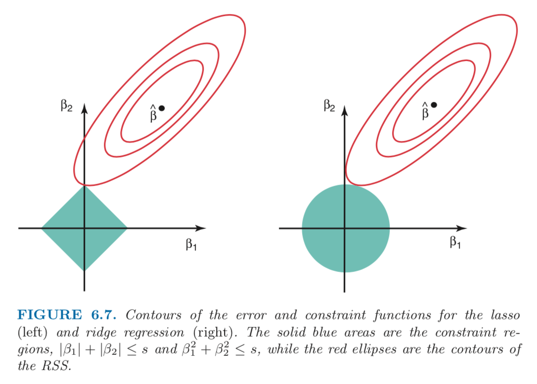
Figure 6.7 illustrates the situation. The least squares solution is markedas $\hat{\beta}$, while the blue diamond and circle represent the lasso and ridge regression constraints in (6.8) and (6.9), respectively. If $s$ is sufficiently large, then the constraint regions will contain $\hat{\beta}$, and so the ridge regression and lasso estimtes will be the same as the least squares estimates. (Such a large value of $s$ corresponds to $\lambda = 0$.) However, in Figure 6.7 the least squares estiamtes lie outside of the diamond and the circle, and so the least squares estiamtes are not the same as the lasso and ridge regression estimates.
The red ellipses that are centered around $\hat{\beta}$ represent regions fo constant $RSS$. In other words, all of the points on a given ellipse share a common value of the $RSS$. Equation (6.8) and (6.9) indicate that the lasso and ridge regression coefficient estimates are given by the first point at which an ellipse contacts the constraint region. Since ridge regression has a circular contraints with no sharp points, this intersection will not generally occur on an axis, and sod the ridge regression coefficient estimates will be exclusively non-zero. However, the lasso constraint has corners at each of the axes, and so the ellipse will often intersect the constraint region at an axis. When this occurs, one of the coefficient estimates may equal zero. In higher dimension, many of the coefficient estimates may equal zero simultaneously.
Comparing the Lasso and Ridge Regression
It is clear that the lasso has a major advantage over ridge regression, in that it produces simpler and more interpretable models that involve only a subset of the predictors. However, which method leads to better prediction accuracy?
Neither ridge regression nor the lasso will universally dominate the other. In general, one might expect the lasso to perform better in a setting where a relatively smally number of predictors have substantial coefficients, and the remaining predictors have coefficients that are very small or that equal zero. Ridge regression will perform better when the response is a function of many predictors, all with coefficients of roughly equal size. However, the number of predictors that is related to the response is never known a prior for real datasets. A technique such as cross-validation can be used in order to determine which approach is better on a particular data set.
As with ridge regression, when the least squares estimates have excessively high variance, the lasso solution can yield a reduction in variance at the expense of a small increase in bias, and consequently can generate more accurate predictions. Unlike ridge regression, the lasso performs variable seleciton, and hence results in models that are easier to interpret.
A simple special case for Ridge Regression and the Lasso
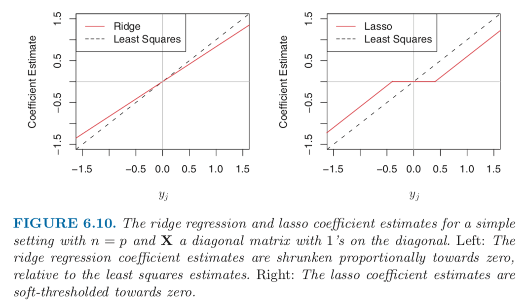
In order to obtain a better intuition about the behavior of ridge regression and the lasso, consider a simple special case with $n = p$, and $X$ a diagonal matrix with 1’s on the diagonal and 0’s in all off-diagonal elements.
To simply the problem further, assume also that we are performing regression without an intercept. With these assumptions, the usual least squares problem simplifies to finding $\beta_1, \ldots,\beta_p$ that minimize
In this case, the least squares solution is given by
And in this setting, ridge regression amounts to finding $\beta_1,\ldots,\beta_p$ such that
is minimized, and the lasso amounts to fiding the coefficients such that
is minimized. One can show that in this setting, the ridge regression estimates take the form
and the lasso estimates take the form
Figure 6.10 displays the situation. We can see that ridge regression and the lasso perform two very different types of shrinkage. In ridge regression, each least squares coeffcient estimate is shrunken by the same proportion. In contrast, the lasso shrinks each least squares coefficient towards zero by a constant amoutn, $\lambda / 2$; the least squares coefficients that are less than $\lambda/2$ in absolute value are shrunked entirely to zero. The type of shrinkage performed by the lasso in this simple setting is known as soft-thresholding.
Bayesian interpretation for Ridge Regression and the Lasso
We now show that one can view ridge regression and the lasso through a Bayesian lens. A Bayesian viewpoint for regression assumes that the coefficient vector $\beta$ has some prior distribution, say $p(\beta)$, where $\beta = (\beta_0, \beta_1,\ldots,\beta_p)^T$. The likelihood of the data can be written as $f(Y|X,\beta)$, where $X=(X1,\ldots,X_p)$. Multiplying the prior distribution by the likelihood gives us the posterior distribution, which takes the form
where the proportionality above follows from Bayes’ theorem, and the equality above follows from the assumption that $X$ is fixed.
We assume the usual linear model,
and suppose that the errors are independent and drawn from a normal distribution. Furthermore, assume that $p(\beta) = \prod_{j=1}^p g(\beta_j)$, for some density function $g$. It turns out that the ridge regression and lasso follow naturally from two special cases of $g$:
If $g$ is a Gaussian distribution with mean zero and standard deviation a function of $\lambda$, then it follows that the
posterior modefor $\beta$ – that is, the most likely value for $\beta$, given the data – is given by the ridge regressioin solution. In fact, the ridge regression solution is also the posterior mean.If $g$ is a double-exponential (Laplace) distribution with mean zero and scale parameter a function of $\lambda$, then it follows that the posterior mode for $\beta$ is the lasso solution. However, the lasso solution is not the posterior mean, and in fact, the posterior mean does not yield a sparse coefficient vector.
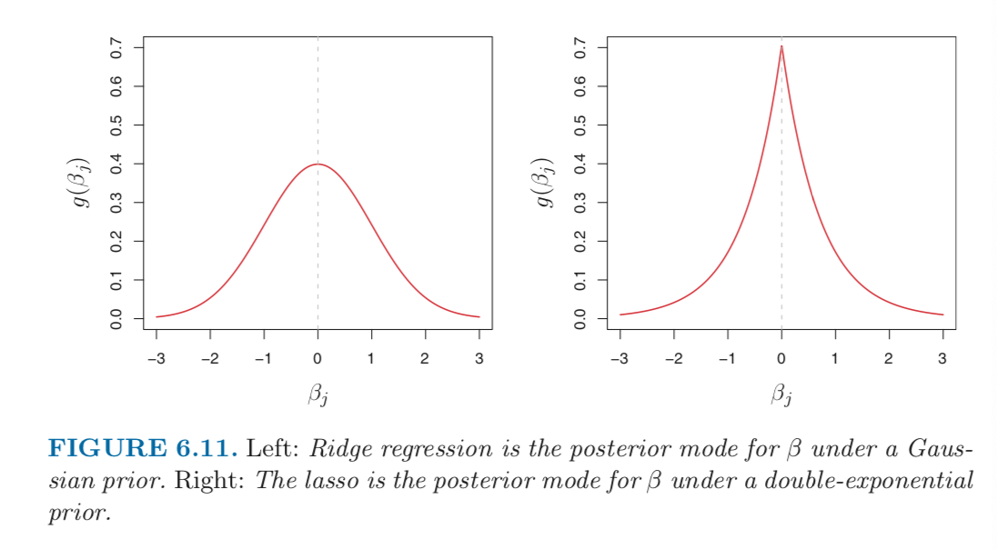
The Gaussian and double-exponential priors are displayed in Figure 6.11. Therefore, from a Bayesian viewpoint, ridge regression and the lasso follow directly from assuming the usual linear model with normal errors, together with a simple prior distribution for $\beta$. Notice that the lasso prior is steeply peaked at zero, while the Gaussian is flatter and fatter at zero. Hence, the lasso expects a priori that many of the coefficients are exactly zero, while ridge assumes the coefficients are randomly distributed about zero.
Selecting the Tuning Parameter
Implementing ridge regression and the lasso requires a method for selecting a value for the tuning parameter $\lambda$ in (6.5) and (6.7), or equivalently, the value of the constraint $s$ in (6.9) and (6.8). Cross-validation provides a simple way to tackle this problem. We choose a grid of $\lambda$ values, and compute the corss-validation error for each value of $\lambda$. We then select the tuning parameter value for which the cross-validation error is smallest. Finally, the model is re-fit using all of the available observations and the selected value of the tuning parameter.
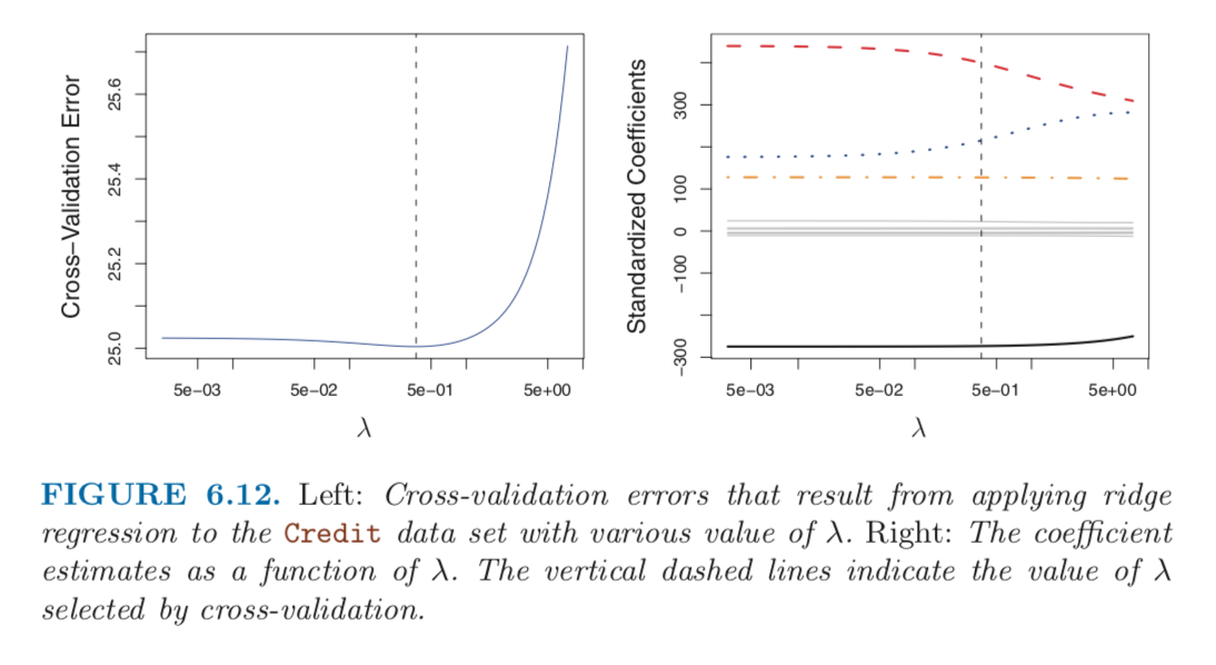
Figure 6.12 displays the choice of $\lambda$ that results from performing leave-out-out cross-validation on the ridge regression fits from the Credit data set.
Dimension Reduction Methods
The methods that we have discussed so far have controlled variance in two differenct ways, either by using a subset of the original variables, or by shrinking their coefficients toward zero. All of these methods are defined using the original predictors, $X_1, X_2, \ldots, X_p$. We now explore a class of approaches that transform the predictors and then fit a least squares model using the transformed variables. We will refer to these techniques as dimension reduction methods.
Let $Z_1,Z_2,\ldots,Z_M$ represent $M < p$ linear combinations for our original $p$ predictors. That is,
for some constants $\phi_{1m},\ldots,\phi_pm$, $m=1,\ldots,M$. We can then fit the linear regression model
using least squares. Note that in (6.17), the regression coefficients are given by $\theta_0,\theta_1,\ldots,\theta_M$. If the constant $\phi$ are chosen wisely, then such dimention reduction approaches can often outperform least squares regression.
The term dimension reduction comes from the fact that this approach reduces the problem of estimating the $p+1$ coefficients to the simpler problem of estimating the $M+1$ coefficients, where $M < p$.
Notice that from (6.16),
where
Hence (6.17) can be thought of as a special case of the original linear regression model given by (6.1). Dimension reduction serves to constrain the estimated $\beta_j$ coefficients, since now they must take the form (6.18). This constraint on the form of the coefficients has the potential to bias the coefficient estimates. However, in situations where $p$ is large relative to $n$, selecting a value of $M \ll p$ can significantly reduce the variance of the fitted coefficients. If $M = p$, and all the $Z_m$ are linear independent, then (6.18) poses no constraints. In this case, no dimension reduction occurs, and so fitting (6.17) is equivalent to performing least squares on the original $p$ predictors.
All dimension reduction methods work in two steps. First, the transformed predictors $Z_1,Z_2,\ldots,Z_M$ are obtained. Second, the model is fit using these $M$ predictors. However, the choice of $Z$ or equivalently, the selection of the $\phi$s, can be achieved in different ways. In this chapter, we will consider two approaches for this task: principal components and partial least squares.
Principal Components Regression
Principal Components Regression (PCA) is a popular approach for deriving a low dimensional set of features from a large set of variables.
PCA is a technique for reducing the dimension of a $n \times p$ data matrix $X$. the first principal component direction of the data is that along which the observation vary the most. For instance, consider Figure 6.14, which shows population size in tens of thousands of people, and ad spending for a particular company for 100 cities. The green solid line represents the first principal component direction of the data. We can see by eye that this is the direction along which tere is the greatest variability in the data. That is, if we project the 100 observations onto this line, then the resulting proejcted observations would have the largest possible variance.
The first principal component is displayed graphically in Figure 6.14, but how can it be summarized mathematically? It is given by the formula
Here $\phi_{11} = 0.839$ and $\phi_21 = 0.544$
are the principal component loadings, which define the direction refered to above. In (6.19), $\overline{\text{pop}}$ indicates the mean of all pop values in this data set, and $\overline{\text{ad}}$ indicates the mean of all ad spending. The idea is that out of every possible linear combinatioin of pop and ad such that
this particular linear combination yields the highest variance.
Since $n = 100$, pop and ad are vectors of length 100, and so is $Z_1$. For instance,
The values of $z$ are known as the principal component score, and can be seen in the right-hand panel of Figure 6.15.
There is also another interpretation for PCA: the first principal component vector defines the line that is as close as possible to the data. For instance, in Figure 6.14, the first principal component line minimizes the sum of the squared perpendicular distances between each point and the line. These distances are plotted as dashed line segments in the left-had panle of Figure 6.15, in which the crosses represent the projection of each point onto the first principal component line. The first principal component has been chosen so that the projected observations are as close as possible to the original observations.
In the right panel of Figure 6.15, the left panel has been rotated so that the first principal component direction coincides with the x-axis. It is possible to show that the first principal component score for the $i$th observation, given in (6.20), is the distance in the x-direction of hte $i$th cross from zero.
We can think of the values of the principal component $Z_1$ as single-number summaries of the join pop and ad for each location. How well can a single number represent both pop and ad? In this case, Figure 6.14 indicates that pop and ad have approximately a linear relationship, and so we might expect that a single-number summary will work well. The first principal component appears to capture most of the information contained in the pop and ad predcitors.
So far we have concentrated on the first principal component. In general, one can construct up to $p$ distinct principal components. The second principal component $Z_2$ is a linear combination of hte variables that is un-correlated with $Z_1$, and has largest variance subject to this constraint. The second principal component direction is illustrated as a dashed blue line in Figure 6.14. It turns out that the zero correlation condition of $Z_1$ with $Z_2$ is equivalent to the condition that the direction muset be perpendicular, or orthogonal, to the first principal component direction.
With two-dimensional data, we can construct at most two principal components. However, if we had other predictors, then additional components could be constructed. They would successively maximize variance, subject to the constraint of being uncorrelated with the preceding components.
The Principal Components Regression Approach
The principal components regression (PCR) approach involves constructing the first M principal components, $Z_1,\ldots,Z_M$, and then using these components as the predictors in a linear regression model that is fit using least squares. The kye idea is that often a small number of principal components suffice to explain most of the variability in the data, as well as the relationship with the response. In other words, we assume that the directions in which $X_1,\ldots,X_p$ show the most variation are the directions that are associated with $Y$. While this assumption is not guranteed to be true, it often turns out to be a reasonable enough approximation to give good results.
If the assumption underlying PCR holds, then fitting a least squares model to $Z_1,\ldots,Z_M$ will lead to better results than fitting a least squares model to $X_1,\ldots,X_p$, since most or all of the information in the data that related to the response is contained in $Z_1,\ldots,Z_M$, and by estimating only $M \ll p$ coefficients we can mitigate overfitting.